Environmental policies and chemicals risk management programmes are essential to protect both human health and the environment from the risks posed by hazardous chemicals. These interventions typically require robust economic justification to demonstrate their necessity and effectiveness. Such justifications often take the form of cost-benefit analyses (CBAs), which assess whether the expected benefits generated by a policy outweigh the costs of policy implementation. The willingness-to-pay (WTP) and value of a statistical case (VSC) values produced by the SWACHE project provide necessary information for calculating these societal benefits. Following a brief overview of the principles of CBA, this chapter highlights the advantages of using SWACHE values in economic impact assessments. It then provides practical guidance on how these values can be applied in CBAs and break-even analyses, illustrated through both hypothetical and real-world examples.
Economic Valuation of Chemicals‑Related Health Effects

Abstract
Cost-Benefit Analysis (CBA) is an assessment method that quantifies all the costs and benefits of a project in monetised terms. In CBA of policies or programmes that improve human health, health benefits are usually first measured in physical terms. For morbidity impacts, benefits are typically quantified as the number of disease cases avoided due to the policy, compared to the status quo. These avoided cases are then monetised by multiplying them by the corresponding value of a statistical case (VSC) of the relevant health effect. A similar logic applies to mortality impacts, where avoided fatalities are monetised using the value of statistical life (VSL) (OECD, 2025[1]). Costs are quantified in terms of all the policy inputs including the net value of labour, materials, and capital used to implement and operate a policy.

Source: Authors’ own elaboration.
As illustrated in Figure 4.1, CBA then consists of comparing the policy costs to the monetised benefits. The difference between the total discounted benefit and the total discounted cost is called the net present value (NPV). If there are several competing policy options, CBA can also be employed to compare them and determine which one has the highest NPV.
To date, a major challenge in policy evaluation and risk management assessment has been a lack of data for valuing the benefits from avoided morbidity outcomes. When WTP values are not available, benefit analyses often rely on qualitative assessments, quantitative but non-monetised metrics, or value approximations, which may in some cases be derived from fractions of mortality values. Among the most common non-monetised metrics for quantifying morbidity effects and making them comparable to mortality impacts are disability-adjusted life years (DALYs) and quality-adjusted life years (QALYs) (see Box 4.1). Due to their non-monetary nature, DALYs and QALYs are not directly suitable for use in CBA. However, under certain assumptions, they can be combined with valuations of statistical life years (VSLY) and converted into monetised units.
WTP and VSC values from the Surveys on Willingness-to-pay to Avoid negative Chemicals-related Health Effects (SWACHE) project enhance the quality of policy impact assessments, by quantifying the intangible welfare benefits associated with reducing or eliminating specific non-fatal health risks associated with chemicals exposure. In particular, the SWACHE valuation approach offers a direct valuation of the health effect which allows for a more transparent and ready-to-use valuation that does not require assessing morbidity as a fraction of mortality or using other approximations. Values from the SWACHE project are therefore convenient for direct application in CBA.
SWACHE values are expressed as VSC whenever the risk reduction in the valuation scenario permits. VSCs are convenient for CBA because they provide a value per case, which can be directly multiplied by the number of cases averted to estimate monetary benefits. Furthermore, VSC estimates also facilitate comparisons across different health outcomes, similar to disability-adjusted life years (DALYs) and quality-adjusted life years (QALYs) measures, as detailed below in Box 4.1.
Since the 1990s, the World Health Organisation (WHO) has produced estimates of disease impacts, most commonly using metrics such as disability-adjusted life years (DALYs) for fatal and non-fatal outcomes for hundreds of diseases and health outcomes. Another common metric developed by academics and health institutions over more than 50 years – the Quality-Adjusted Life Years (QALY) – also establishes a single metric for fatal and non-fatal outcomes.
DALYs are a measure of the overall burden of disease, expressing the number of years lost due to ill-health, disability or premature death. For a given disease, DALYs are the sum of years lived with disability (YLDs) and the years of life lost (YLLs). To estimate YLDs for a particular cause in a particular time period, the number of incident cases in that period is multiplied by the average duration of the disease and a weight factor that reflects the severity of the disease on a scale from 0 (perfect life) to 1 (dead). Disability weights are determined using input from medical experts and the general population. To estimate YLLs attributable to a particular cause (such as chemicals exposure), the number of cause-specific deaths are multiplied by a loss function specifying the years lost for deaths as a function of the age at which death occurs.
QALYs combine information on quality and quantity of life generated by healthcare interventions. QALYs weight each year of life by a health-related quality-of-life score ranging from 0 (death) to 1 (perfect health). One QALY is equal to one year in perfect health.
DALYs and QALYs are both utility metrics that integrate considerations of health and longevity. They can be used in Cost-Effectiveness Analysis (CEA), where the benefits are measured in “years” and costs in monetised units. CEAs are often used in the field of health services to inform resource allocation and compare different health gains. In the absence of robust WTP estimates tailored to a specific condition, such as those derived from the SWACHE project, other approaches – such as monetised QALYs or DALYs or cost-of-illness (COI) methods – can be used as approximations in CBA depending on the policy problem assessed (Robinson et al., 2019[2]; Herrera-Araujo et al., 2026[3]).
However, these approaches have limitations. COI estimates are often underestimates of WTP measures, as they do not capture the disutility of illness and estimates of WTP per QALY rely on strong assumptions about the valuation of health states over time and how health changes are experienced across the life course (Gyrd-Hansen, 2005[4]).
The Global Burden of Disease (GBD) study, led by the Institute for Health Metrics and Evaluation (IHME) in collaboration with governments and academic institutions around the world, regularly reports mortality and morbidity data for causes of death, diseases, injuries, and risk factors, including disability‑adjusted life years (DALYs) and associated disability weights. While the SWACHE project provides an economic perspective on health benefit measures, policymakers can use complementary data from the GBD, for example, to determine baseline levels of mortality and morbidity in a population. When available and where comparisons were possible, the disability weights of the health effects addressed in SWACHE were compared with the VSC ranking shown in Figure 2.1 of Chapter 2. The comparison appears broadly consistent. For instance, “stage 3 chronic kidney disease” has a higher disability weight than “symptomatic hypothyroidism”, which in turn has a lower disability weight than “partially controlled asthma”, consistent with the VSC ranking (IHME, 2023[5]). This comparison is not exhaustive and indicative only, as some endpoints are not labelled or defined similarly in the SWACHE and GBD datasets. For example, hypertension is primarily classified in the GBD as a risk factor or a cause of other diseases rather than as a health state in itself.
As discussed earlier, the first two rounds of the SWACHE project provide WTP and VSC estimates for ten health effects. These values can be readily combined with estimated policy impacts, which are typically firstly expressed as the number of cases avoided or increased by the introduction or removal of a given policy under consideration. In the context of a policy aiming at improving quality of life and reducing negative health outcomes, the associated economic benefits can be calculated by multiplying the number of cases avoided by the corresponding WTP or VSC value. The methodology for applying VSC estimates is detailed below, and a similar approach applies to WTP estimates.
The first step is to adjust the nominal VSC estimate for inflation and growth in income over time to reflect its value in the year of use. These adjustments reflect the relationship between income levels and individuals’ WTP, as highlighted in Table 3.1 of Chapter 3. While Gross Domestic Product (GDP) per capita1 is a commonly used approximation of income growth, countries may also prefer alternative indicators that better align with national context and practices, such as household annual or weekly earnings or median income growth. Inflation can be measured using changes in the Consumer Price Index (CPI).
The second step is to calculate the benefits of the policy by multiplying the updated VSC by the number of cases prevented every year by the policy. In a retrospective policy evaluation, the number of cases prevented by the policy can be estimated by comparing the actual number of cases in the population before and after the policy was implemented, while remaining cautious that not all avoided cases are necessarily directly attributable to the policy. In a prospective policy appraisal, the number of cases to be prevented depends on the objectives set for the policy. Alternatively, a break-even analysis can be performed, in which the VSC estimates are used to determine the number of avoided cases needed to offset the costs of the policy, as detailed in the section below.
Importantly, the time lag between changes in exposure to chemicals and the onset of associated health effects should be considered. Some acute effects can be immediate, such as skin irritation, while for other health endpoints this time lag can extend over days, months, or even years. Additionally, some effects may also result in mortality, posing challenges for both epidemiology and valuation. Understanding this time lag can inform how to appropriately account for the total benefits of policies that restrict certain chemicals.
Finally, annual benefits of the policy should be discounted with respect to the base year and then summed across years. The OECD recommends that the discount rate used should follow national government guidance on discount rates for cost-benefit analysis. For example, the United Kingdom government recommended a 1.5% discount rate for health and risk impacts in 2022 (UK Government, 2022[6]). The European Commission’s Better Regulation Toolbox recommended in 2023 a 3% discount rate for EU policy analysis (European Commission, 2023[7]). These rates are typically revised periodically.
Table 4.1 provides an illustrative example of how the methodology detailed above can be applied based on a hypothetical policy that is expected to reduce the number of cases of miscarriage by 1 000 every year in France for 2023-2026. Based on a mean VSC of USD2023 325 235 (i.e. EUR2023 216 673), the discounted benefits from the policy over the 4 years equal EUR2023 858 million.
Note: This illustrative example assumes a fictional policy that would reduce the number of statistical cases of miscarriage by 1 000 every year in France from 2023 to 2026. GDP per capita figures and projections come from the OECD Economic Outlook (OECD, 2025[8]) and the OECD Dataset Population projections as of July 2025. Consumer Price Index data for 2023 comes from the OECD Dataset: Consumer price indices as of September 2025. A 2% increase per year is assumed for the Consumer Price Index for 2024-2026 and is not an OECD forecast. PPP for actual individual consumption data is for year 2023 and come from the OECD Dataset: Annual Purchasing Power Parities and exchange rates as of September 2025. The discount rate is based on the ECB figures. (European Central Bank, 2025[9]). The income elasticity equals 0.26 as estimated in the working paper (Dockins et al., 2026[10]).
Similarly, WTP values from the asthma severity survey and the IQ loss in children survey are useful for CBAs. In the IQ loss survey, the reported WTP refers to the amount individuals are willing to pay to avoid the loss of one IQ point in a hypothetical child. Therefore, this WTP can be adjusted for inflation and GDP per capita and then multiplied by the number of IQ points that the policy would prevent from being lost. For example, if a fictional policy avoids the loss of 1 IQ point among 6 000 children born between 2022 and 2027, the resulting discounted benefits would be USD2022 21 million in the United States and about USD2022 20 million (i.e. DKK2022 147 million) in Denmark. These results are obtained using a 3% discount rate for the United States and a 4% discount rate for Denmark (Mourato et al., 2023[11]).
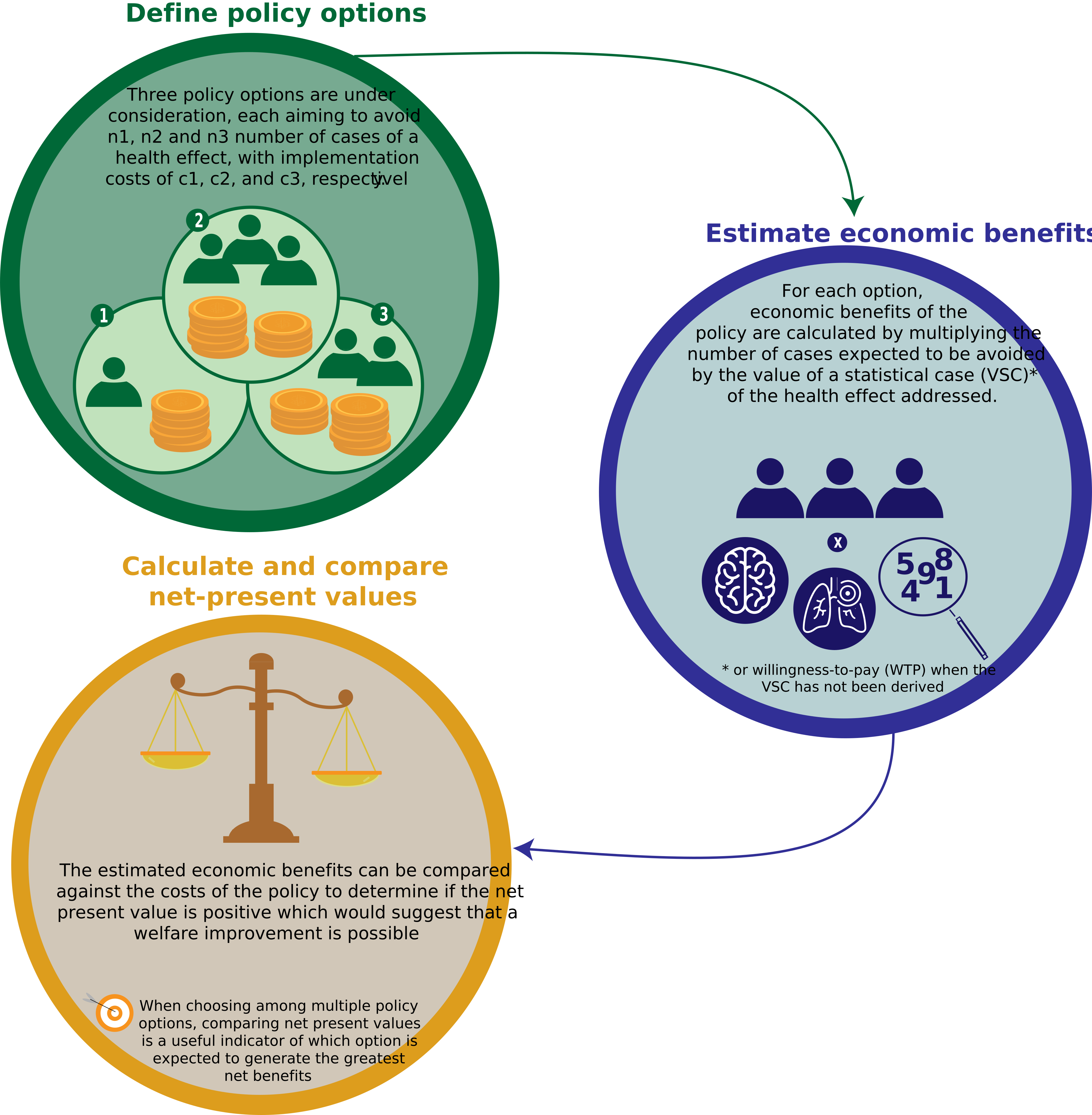
In the context of health policies or chemicals management programmes, the evaluation of benefits and costs often requires comparing impacts that occur in different time periods, for example in cases where there is a latency period between exposure reduction and the occurrence or avoidance of health effects. Analysts and policymakers can address these timing differences by applying discounting to reflect time preferences, following best practice or standard guidance on the choice of discount rate from national or international CBA guidelines (Robinson and Hammitt, 2011[12]; OECD, 2025[1]). Figure 4.2. summarises and illustrates the steps leading to the comparison of policy costs and benefits, as well as the comparison across different policy options.
A point of discussion concerns how WTP/VSC estimates should be considered in relation to other health benefit or avoided cost estimates. As explained in Section 1.5 of Chapter 1, the WTP estimates of the SWACHE project reflect the broad physical, emotional, social and economic burden of disease. Consequently, adding these estimates to other metrics such as cost-of-illness (COI) may entail a risk of double-counting, since the WTP/VSC already reflects avoided health care expenditures and productivity losses as perceived and anticipated by individuals when reporting their WTP (Drummond et al., 2015[13]; DEFRA UK, 2025[14]). The asthma survey constitutes an exception, as respondents were explicitly instructed to ignore monetary costs when stating their WTP. In this specific case, combining WTP estimates with COI measures may be considered. Nevertheless, despite asking respondents to focus only on the non-monetary benefits, 40% of respondents reported in the debriefing questions of the asthma survey that they had anticipated medical cost savings (Appéré et al., 2023[15]). This share reaches 60% in the United States. This finding supports the use of WTP as a measure capturing the full welfare benefits of reducing the risk of developing or worsening a disease, as perceived by individuals (Nocera, Telser and Bonato, 2003[16]).
As illustrated in Figure 4.2., VSC and WTP values can be used to calculate the benefits of the policy option. Conversely, since the benefits equal the VSC multiplied by the number of cases avoided, VSC estimates can also be used to demonstrate the number of cases that must be avoided for the policy benefits to offset its implementation costs. Such analyses are called break-even analyses and consist of determining how many cases of a given illness would need to be avoided to economically justify a policy intervention. Similarly, in the context of comparing or switching between options, switching cost analyses can be performed to assess whether the additional benefits from a new option are sufficient to justify the additional costs of switching from a previous option. The number of cases that would need to be avoided in the population for the intervention to break even can be compared with the number of cases actually observed in the same population. The intervention is likely to be justified where the required number of avoided cases is lower than the actual number of avoided cases observed or predicted.
In 2025, the United Kingdom strengthened its chemicals regulation of Persistent Organic Pollutants (POPs) using SWACHE values as inputs for a switching costs analysis (DEFRA UK, 2025[14]). POPs are toxic substances that accumulate in living organisms and pose significant health risks that could include a number of health effects. The impact assessment of the amendment intended to strengthen the regulation included a switching cost analysis, which used SWACHE values for chronic kidney disease, infertility and very low birth weight to compare the health benefits against the business costs of the regulation. The impact assessment estimated that between 83 and 119 incidences of these diseases need to be avoided to offset the estimated regulatory extra costs of £68 million (~EUR 78 million).
Note: This switching cost analysis aggregates the different values by taking the simple average of the values of the four diseases considered. The total costs of the regulation were then divided by this averaged value of a statistical case in order to derive the incidences of the diseases that need to be avoided to offset these costs. This approach is presented here to illustrate the methodology of the break-even analysis, consisting of dividing the costs by the value of a statistical case of a disease to derive the incidence of disease that needs to be avoided to offset the costs. However, the methodology used to calculate the average value across the four diseases is not the recommended OECD approach. The discussion on the valuation of multiple health effects is provided in Chapter 6.
Source: 2025 Amendments to the Persistent Organic Pollutants Regulations, Annexes I, IV and V, covering two Statutory Instruments (DEFRA UK, 2025[14]).
In addition to the United Kingdom Government’s impact assessment mentioned above, SWACHE values are also used by multiple institutions. The European Chemicals Agency (ECHA) updated its reference values in September 2023 to monetise the health impacts of chemicals, using VSC estimates derived from the SWACHE project for infertility, adult and childhood asthma, chronic kidney disease, and very low birth weight (ECHA, 2023[17]) and updates for other SWACHE endpoints are envisaged in the near future. These reference values are used by ECHA for applications for authorisation and restriction dossiers concerning substances that pose a risk to human health and the environment. In a similar vein, the European Commission considers the SWACHE project for methodological aspects related to the costing of chemical pollution for our society (European Commission, 2026[18]). Finally, SWACHE values are also used as contextual evidence in discussions and international conventions, such as the Rotterdam Convention, which addresses hazardous chemicals and pesticides in international trade (UNEP/FAO, 2025[19]).
References
[15] Appéré, G. et al. (2023), “Valuing a reduction in the risk and severity of asthma: A large scale multi-country stated preference approach”, OECD Environment Working Papers, No. 218, OECD Publishing, Paris, https://doi.org/10.1787/f289d29e-en.
[14] DEFRA UK (2025), Title: 2025 Amendments to the Persistent Organic Pollutants Regulations, Annexes I, IV and V, covering two Statutory Instruments.
[10] Dockins, C. et al. (2026), “Valuing a reduction in the risk of miscarriage: A large-scale multi-country stated preference approach”, OECD Environment Working Papers, No. 271, OECD Publishing, Paris, https://doi.org/10.1787/23bb6643-en.
[13] Drummond, M. et al. (2015), Methods for the Economic Evaluation of Health Care Programmes, Press, Oxford University, https://nibmehub.com/opac-service/pdf/read/Methods%20for%20the%20Economic%20Evaluation%20of%20Health%20Care%20Programmes.pdf.
[17] ECHA (2023), Reference willingness-to-pay values for monetising chemicals health impacts, https://echa.europa.eu/documents/10162/17229/seac_reference_wtp_values_en.pdf/b041ac3c-5874-76fc-f317-84cf565c8f7b.
[9] European Central Bank (2025), Monetary policy decisions, https://www.ecb.europa.eu/press/pr/date/2025/html/ecb.mp250911~6afb7a9490.en.html.
[7] European Commission (2023), Better regulation toolbox 2023, https://commission.europa.eu/document/download/0d32ee11-92da-434d-9c86-fd4579d95dc6_en?filename=BRT-2023-Chapter%208-Methodologies%20for%20analysing%20impacts%20in%20IAs%20evaluations%20and%20fitness%20checks_0.pdf.
[18] European Commission, D. (2026), The cost of PFAS pollution for our society, https://data.europa.eu/doi/10.2779/9590509.
[4] Gyrd-Hansen, D. (2005), “Willingness to Pay for a QALY”, PharmacoEconomics, Vol. 23/5, pp. 423-432, https://doi.org/10.2165/00019053-200523050-00002.
[3] Herrera-Araujo, D. et al. (2026), WTP for fatal and non-fatal environmental related disease: a QALY-based study across Europe, https://valesor.eu/download/18.9ea4e0e19c47c9d0a82b0cf/1771840198009/WTP-for-Fatal-and-Non-Fatal-Environmental-Related-Diseases.pdf.
[5] IHME (2023), GBD Results, Institute for Health Metrics and Evaluation, https://vizhub.healthdata.org/gbd-results/.
[11] Mourato, S. et al. (2023), “Valuing the avoidance of IQ losses in children: A large scale multi-country stated preference approach”, OECD Environment Working Papers, No. 219, OECD Publishing, Paris, https://doi.org/10.1787/71574eb4-en.
[16] Nocera, S., H. Telser and D. Bonato (2003), “Cost-Benefit Analysis”, in Developments in Health Economics and Public Policy, The Contingent Valuation Method in Health Care, Springer US, Boston, MA, https://doi.org/10.1007/978-1-4419-9133-1_8.
[1] OECD (2025), Mortality Risk Valuation in Policy Assessment: A Global Meta-Analysis of Value of Statistical Life Studies, OECD Publishing, Paris, https://doi.org/10.1787/76ca89a2-en.
[8] OECD (2025), OECD Economic Outlook, Volume 2025 Issue 1: Tackling Uncertainty, Reviving Growth, OECD Publishing, Paris, https://doi.org/10.1787/83363382-en.
[12] Robinson, L. and J. Hammitt (2011), “Behavioral Economics and the Conduct of Benefit-Cost Analysis: Towards Principles and Standards”, Journal of Benefit-Cost Analysis, Vol. 2/2, pp. 1-51, https://doi.org/10.2202/2152-2812.1059.
[2] Robinson, L. et al. (2019), “Conducting Benefit-Cost Analysis in Low- and Middle-Income Countries: Introduction to the Special Issue”, Journal of Benefit-Cost Analysis, Vol. 10/S1, pp. 1-14, https://doi.org/10.1017/bca.2019.4.
[20] Robinson, L., J. Hammitt and L. O’Keeffe (2019), “Valuing Mortality Risk Reductions in Global Benefit-Cost Analysis”, Journal of Benefit-Cost Analysis, Vol. 10/S1, pp. 15-50, https://doi.org/10.1017/bca.2018.26.
[6] UK Government (2022), The Green Book, https://www.gov.uk/government/publications/the-green-book-appraisal-and-evaluation-in-central-government/the-green-book-2020#a6-discounting.
[19] UNEP/FAO (2025), Conference of the Parties to the Rotterdam Convention on the Prior informed consent procedure for certain hazardous chemicals and pesticides in international trade, United Nations Environment Programme/Food and Agriculture Organization of the United Nations, https://www.pic.int/Portals/5/download.aspx?d=UNEP-FAO-RC-COP.12-INF-18.En.docx.
← 1. GDP per capita is used in this report and the SWACHE working papers, in line with common practices in cost‑benefit analysis (CBA) which frequently relies on GDP per capita or Gross National Income (GNI) as approximations for income growth (Robinson, Hammitt and O’Keeffe, 2019[20]; OECD, 2025[1]).