Commuting data provide valuable information on labour-market relationships, but work accounts for only part of people’s daily mobility. Trips made to access education, healthcare, shops, services, leisure and social activities also shape the territories within which people conduct their everyday lives. Mobile phone data can complement official commuting statistics by capturing a wider range of trip purposes at greater spatial and temporal detail. They can therefore help assess whether rural daily systems reflect broader patterns of mobility rather than journeys to work alone. This chapter examines the opportunities and limitations of using mobile phone data to analyse rural daily systems. It draws on cell-tower-based data provided by the Korea Transport Institute and GPS-based data supplied by Habidatum for Australia, Canada, Japan and the United Kingdom. The chapter evaluates their territorial coverage, compares mobile-derived commuting flows with official sources and examines how well FRAs combined with FUAs capture work and non-work trips. It also compares their performance with LMAs in Japan and Australia. The analysis provides new evidence on the geography of everyday mobility, while also highlighting the need to account for uneven user coverage, particularly in remote areas.
The Geography of Choice

Abstract
Mobile phone data is a general term used to indicate any georeferenced data that is generated through the use of mobile phone devices. Mobile phone data can usually be of two types:
Cell-tower-based data (Mobile Network Operator – MNO – data or network data): Generated by the mobile phone devices interacting with the mobile network and leaving temporal and geographical signatures accessible to Mobile Network Operators (MNOs). These data come from logs to the cell tower that a mobile device connects to when making a call, sending a text, or simply being active on the network. They provide broad population coverage and long timeframes. The spatial accuracy of these data depends on density of cell towers and coverage area of each tower.
GPS-based data (app or device data): Generated by the mobile phone devices interacting with mobile applications (apps) that use the GPS functionality to provide services such as navigation, location-based recommendations, or geotagging. Compared to MNO data, GPS data potentially provide higher spatial and temporal accuracy in detecting mobility patterns. On the other hand, the representativeness of GPS data depends on its sample size, which may be limited.
Mobile phone data have the potential to reveal high-frequency, multi-purpose mobility patterns at fine spatial scale across the entire urban-rural gradient. Compared to census-based commuting flows, mobile phone data have the potential to observe multiple trip purposes beyond home-to-work trips (e.g. access to services, shopping and leisure), capture temporal dynamics with daily or hourly frequency, and rely on longer observation time periods than a specific survey period or multi-annual snapshot.
The availability and processing of mobile phone data may also present challenges: data acquisition may be costly and reliant on third-parties, including app companies, data brokers and MNOs; signals are noisy and require inference, such as home/work detection, and trip segmentation; spatial accuracy may be uneven, especially tower-based in sparsely-covered areas; and samples may be biased by device ownership, app usage, operator market share and user behaviour. Data samples may under-represent specific population groups, such as older, lower-income, privacy-concerned, or population living in areas with weak coverage. Overall, careful preprocessing, validation and appropriate data weighting are essential.
This section presents an overview of the quality of mobile phone data for a selection of countries, by comparing them to official census or survey data.
Korean Transport Institute (KOTI) mobile phone data
The Korean Transport Institute (KOTI) made available cell-tower based mobile phone data. The dataset provides the number of trips between origin and destination at the hourly level and at 500 m spatial resolution. It covers 13 days that represent different time periods:
2022/10/19, a typical workday
2022/11/07 to 2022/11/13, a typical work week
2022/09/08 to 2022/09/12, Chuseok holiday in Korea.
The KOTI dataset allows analysis of different trip purposes, as it classifies stay points1 into: home, company (work), school, regular potential stay, other potential stay and other. Each flow at the 500 m grid-level is characterised by the corresponding average travel time and distance. Annex C provides details on the preprocessing steps applied by KOTI on the raw mobile-phone data.
Quality assessment
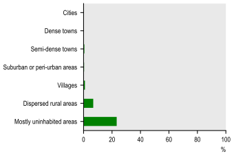
KOTI data exhibit a relatively low share of missing observations. At the municipal level (shi-gun-gu, 시군구), all units record at least one trip and at the sub-municipal level (eup-myeon-dong, 읍면동), only 90 out of 3 504 units are not identified as the origin of any trip. At the grid level, 11.7% of grids cells register no trip origins. In terms of settlement typology, coverage is high across all settlement types, except for dispersed rural areas and largely uninhabited zones, where 7% and 23% of cells, respectively, are not the origin of any trip (Figure 4.1).
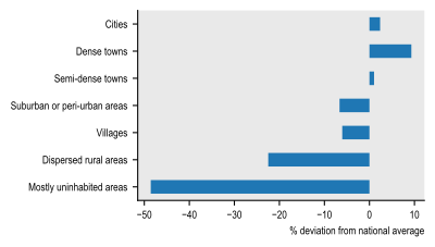
When comparing the distribution of the number of trips and of the resident population across settlements, both show a similar pattern, with trips occurring in proportion to population size (Figure 4.2).
Share of 500 m grid cells that are not the origin of any trip, by degree of urbanisation (level 2)
Source: OECD computations based on KOTI mobile phone data.
Note: Numbers weighted by population.
Work trips per capita by degree of urbanisation (level 2), % deviation from national average
Source: OECD computations based on KOTI mobile phone data.
Note: Trips are classified according to the degree of urbanisation of their points of origin.
However, the distribution of intra- and inter-municipal work-related trips differs from the census-based commuting flows produced by the Korean Statistical Information Service (KOSIS). While KOSIS reports 65.8% of commuters travelling within the same municipality, KOTI data indicate a lower share of 45.7% (Table 4.1).
Source: OECD computations based on KOTI and KOSIS commuting flow data. For KOTI, the commuting flows correspond to typical working days (observed period: 7 to 11 November 2022).
The commuting matrix derived from mobile phone data is then compared with the census-based commuting matrix at municipal level using weighted cosine similarity, a measure that assesses how similar the spatial patterns of commuting flows are while remaining unaffected by differences in total trip volumes. Cosine similarity is a measure of proximity between two non-zero vectors and defined as the dot product of the vectors divided by the product of their magnitude:
where and are the i-thcomponents of vectors and . The cosine similarity ranges from (exactly opposite) to (identical) with indicating perfect orthogonality between the two vectors. Since commuting flows cannot be negative, in our case it ranges from 0 to 1. The global cosine similarity is computed as the population-weighted mean of the individual cosine similarities obtained in each municipality. The global cosine similarity between the KOTI and KOSIS commuting flow matrices is high, reaching 0.94 when weighted by population. The similarity is slightly lower in cities (0.93) but remains close to 0.99 across all other settlement types. This variation likely reflects differences in territorial extent of Korean municipalities, which are relatively small in urbanised contexts (cities) but much larger in less dense areas. Cell-tower-based mobile phone data may also introduce positional uncertainty compared with GPS-based datasets, contributing to small discrepancies in commuting flow patterns, especially where municipalities are small.
Descriptive statistics
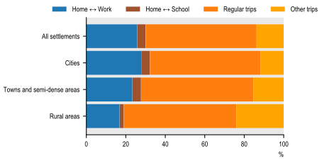
Over a typical work week (7 to 13 November 2022), work-related trips accounted for around 26% of all trips and school-related for a further 2%. Most recorded mobility was therefore associated with other purposes, such as access to services, shopping and leisure. The share of work-related trips also varied significantly across settlement types, from around 28% in cities to 23% in towns and semi-dense areas and 17% in rural areas. These patterns suggest that work commuting represents a smaller proportion of observed mobility in rural areas than in more densely populated settlements. This may reflect more dispersed employment patterns and the importance of trips made to access services and meet other daily needs. The results underline the importance of looking beyond home-to-work flows when analysing rural daily systems (Figure 4.3).
Distribution of trips by type of trip, degree of urbanisation over a typical work week (7 to 13 November 2022)
Source: OECD computations based on KOTI mobile phone data.
Note: Regular trips refer to trips between company, home, school and regular potential stays that are not Home ↔ Work or Home ↔ School. Trips are classified based on the degree of urbanisation and proximity to FUA of their point of origin, based on a 500 m grid.
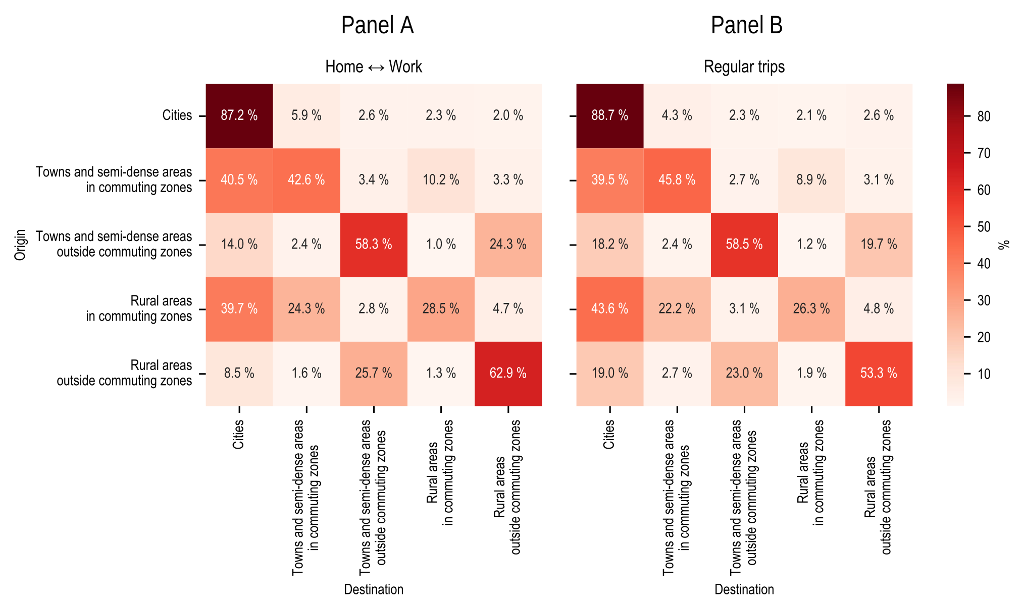
Rural areas outside commuting zones exhibit mobility patterns that differ markedly from those of denser settlements. Figure 4.4 shows the origin-destination matrices derived from mobile phone data, distinguishing between home to work trips (panel A) and regular trips (panel B). Rural areas outside commuting zones are largely self-contained, with almost 63% of work trips originating and ending within those areas. Conversely, 26% of work trips originating in rural areas outside commuting zones are to towns and semi-dense areas outside commuting zones. Very few work trips originating in rural areas outside commuting zones go to cities (9%). Regarding regular trips, a much higher share of people in rural areas outside commuting zones travel to cities (19%). The average travel distances differ considerably across types of settlements and types of trips (Figure 4.5). While work trips in rural areas are comparable to other types of settlements, regular and other trips are longer, indicating that residents must travel further to access services and leisure. This pattern reveals a dual dynamic: economic activity and employment are locally self-contained, yet everyday life remains dependent on urban and regional centres. In contrast, rural areas within commuting zones show that both work- and services-related trips are centred around cities with longer distances for work but shorter for regular trips.
Distribution of home-work and regular trips by degree of urbanisation and proximity to FUAs of their origin and destination stay points over a typical week (7 to 13 November 2022)
Source: OECD computations based on KOTI mobile phone data.
Note: Regular trips refer to trips between company, home, school and regular potential stay that are not Home ↔ Work or Home ↔ School. Calculations are performed at the 500 m grid level.
Average travel distance by type of trip, by degree of urbanisation over a typical week (7 to 13 November 2022)
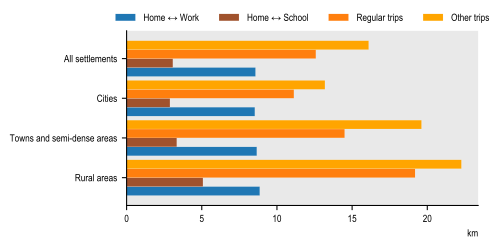
Source: OECD computations based on KOTI mobile phone data.
Note: Regular trips refer to trips between company, home, school and regular potential stay that are not Home ↔ Work or Home ↔ School. Trips are classified based on the degree of urbanisation of their point of origin. Calculations are performed at the 500 m grid level.
Habidatum mobile phone data
A second mobile phone dataset was acquired from Habidatum, a private company specialising in the provision and processing of geolocation data. The dataset covers work- and non-work-related trips for Australia, Canada, Japan and the United Kingdom over the period 2021-2024, at both municipal and 1 km grid-cell level (Table 4.2). It is derived from anonymised GPS location records collected through software development kits (SDKs) embedded in mobile applications providing services such as weather forecasts, navigation, fitness tracking and social media. Data were collected only from users who consented to share their location information. Observations from different applications are combined at the user level and duplicate records are removed.
Approximately 90% of signals are generated while an application is actively in use (foreground). During these periods, a device typically records one location approximately every 5 seconds, although only within relatively short windows, such as during a journey or an errand. The remaining 10% observations are collected passively in the background, generally at intervals of 15 to 60 minutes depending on application permissions and device settings. Recording becomes less frequent when a device remains stationary for an extended period, including overnight, or while a user is at work, and fall to around one observation per hour. Despite the lower density, these background signals remain sufficient to identify regularly visited locations (anchor points), including probable home and workplace locations.
Before trips are identified, the raw observations undergo several cleaning and quality-control steps. Records with invalid coordinates, missing or implausible timestamps, malformed information or non-location diagnostic events are removed. Habidatum retains location estimates derived from the device, including satellite, Wi-Fi and cellular positioning, while excluding less reliable sources such as IP-based geolocation and registration pings. Further filters exclude observations with implausible speeds above 150 km/h, horizontal accuracy poorer than 100 metres or unusual concentrations of signals.
The cleaned observations are then grouped into clusters representing periods during which a device remained in approximately the same location. Habidatum applies the DBSCAN clustering method, using a radius of 150 metres and a minimum duration of 50 seconds. The resulting clusters are classified either as stay points, where a device remained for at least 50 seconds, or as movement events.
Home and work locations are identified from the stay-point history of each device. Home is inferred as the most frequently observed night-time stay point between 22:00 and 08:00, while the workplace is inferred from frequently observed daytime stays between 12:00 and 17:00. Each device is assigned one home and one workplace, and devices for which no home location can be identified are excluded. Other destinations are identified when the device remains at a stay point for more than 30 minutes.
Trips are reconstructed from these inferred locations using an anchor-to-anchor methodology. This means that the dataset does not require continuous observation of the route: a trip can be identified when sufficient information is available at its origin and destination. To improve data quality, Habidatum applies additional rules to simplify trip chains and remove potentially unreliable observations. Trajectories with implausible speeds, statistical outliers or durations exceeding 24 hours are excluded. Home-work-home sequences are recorded as a single commute, intermediate stops lasting less than 30 minutes are ignored, and for journeys involving several destinations, each destination is linked to the home location; for example, a sequence from A to B to C to D is represented by the origin-destination pairs A–B, A–C and A–D.
Source: Habidatum
To produce municipal origin-destination matrices from the grid-level mobility data, Habidatum applied five additional steps:
1. Calculate distances at grid level. Geodesic distances were calculated between the centroids of the 1 km origin and destination grid cells, deriving a metric. This retained information on trip distances before flows were aggregated to municipalities.
2. Assign trips to municipalities. Grid-based origins and destinations were matched to municipal boundaries using a point-in-polygon spatial join. The resulting flows were then aggregated by origin and destination municipality, and average distances were calculated using the number of trips as weights.
3. Construct a population-calibration factor (). GPS-based estimates of residential population were compared with municipal census populations. Where population data from the latest census were unavailable, values from earlier census editions were used.
4. Limit the influence of extreme values. The was winsorised by capping values at the 1st and 99th percentiles.
5. Adjust municipal trip totals. Outbound trips from each municipality were rescaled using the winsorised . This adjustment was intended to make the spatial distribution of the mobile-phone sample more representative of the census population.
Quality assessment
The quality of the Habidatum data varies somewhat across settlement types (Figure 4.6). In all countries, except the UK, cities, towns and suburbs have relatively few grid cells without observed trip origins, while data gaps become more common in less densely populated settlements. In Canada and Japan, for example, more than 20% of 1 km grid cells in villages are not the origin of any trips. Work trips per capita follow a similar pattern: cities consistently record more trips relative to their population than other settlement types, indicating a slight bias towards denser, more populated areas.
Panel A. Share of 1 km grid cells which are not origin of any trip by degree of urbanisation (level 2)

Note: Trips are classified according to the degree of urbanisation of their point of origin.
Source: OECD computations based on Habidatum mobile phone data.
The share of inter- and intra-municipal flows differs from official census-based commuting flows (Table 4.3). In Canada, GPS data show that almost 80% of workers commute within their municipality of residence, compared with around 60% in the census data. In Japan, the pattern is reversed: approximately 47% of work trips remain within the municipality in the GPS data, compared with approximately 56% in the census. The share of municipalities that are not the origin of any work commuting trip is also smaller with census-based commuting flows than with mobile-phone based ones.
Source: OECD computations based on Habidatum mobile phone data, and Statistics Japan and Statistics Canada census-based commuting flows
Note: Commuting flow matrices in Australia are not publicly available.
Despite these differences, the overall geographical pattern of commuting destinations is highly consistent across the two sources. The global cosine similarity index between the mobile-phone and census commuting matrices at municipal level is very high in both Japan (0.96) and Canada (0.93), where a value of 1 indicates identical distributions of commuting flows. Similarity is generally higher in cities than in less densely populated settlements. In Canada, for example, the average cosine similarity ranges from 0.773 in dispersed rural areas to 0.957 in cities. This may be related to the high spatial accuracy of GPS-data compared to cell-tower based data and by the low user coverage in remote areas, which make the resulting origin-destination patterns more sensitive to individual observations.
Population-weighted mean cosine similarity index by degree of urbanisation (level 2) in Canada and Japan
Note: Trips are classified according to the degree of urbanisation of their municipality of origin. No census-based commuting flow data are publicly available for Australia.
Source: OECD computations based on Habidatum mobile phone data, Statistics Canada and e-Stat census-based commuting flows
Given the relatively high share of missing observations in the UK mobile phone data (Figure 4.6), the UK is excluded from the remainder of the analysis. The UK results are nevertheless broadly consistent with those reported for the other countries and are available from the OECD upon request.
Descriptive statistics
The distribution of trips across countries and settlement types reveals distinct patterns. In Canada, almost 14% of trips are work-related, compared with almost 9% in Japan and 5.5% in Australia. The distribution of trips by degree of urbanisation is homogeneous in Australia and in Japan, while in Canada the share of work-related trips is lower in rural areas than in other settlement types (Figure 4.7).
Share of work-related trips, degree of urbanisation
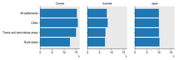
Source: OECD computations based on Habidatum mobile phone data.
Average trip distances exhibit more variation across settlement types (Figure 4.8). Rural areas consistently record the longest trips: in both Canada and Australia, rural residents travel farthest for both work and non-work purposes. In Canada in particular, residents of rural areas travel roughly 2-3 times further for both home-work and home-other trips compared to cities. While Japan displays shorter overall trip distances, it still shows a clear gradient where trips in rural areas are longer than in cities. Across all three countries, non-work trips tend to be slightly longer than journeys between home and work. These results refer to distance travelled rather than travel time. They therefore do not establish that rural residents systematically spend more time travelling. Travel duration also depends on factors such as transport mode, road conditions and congestion, which may substantially increase journey times in more densely populated areas. Longer rural distances may or may not translate into longer travel times.
Average trip distance by type of trip, degree of urbanisation
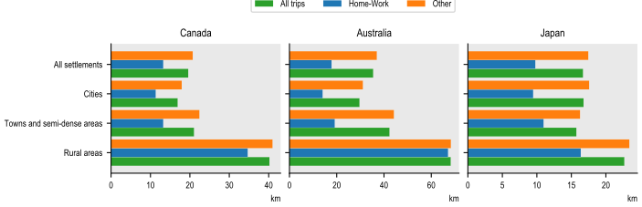
Source: OECD computations based on Habidatum mobile phone data. These results are not driven by outliers.
As introduced in Chapter 3, Martínez-Bernabeu, Coombes and Casado-Díaz (2019[1]) identify four properties to evaluate LMAs: autonomy, cohesion, homogeneity and balance.
1. Autonomy (self-containment): Maximise trips that start and end within the same daily system; too many cross-boundary trips signal misdrawn areas. Given that autonomy can only increase when combining daily systems, it is a useful criterion but cannot stand alone.
2. Cohesion (internal connectivity): Favour strong interaction intensity between local areas belonging to the same daily system. Adding weakly linked places lowers cohesion and counterbalances the push toward ever-larger systems.
3. Homogeneity (similar size): Aim for daily systems of comparable size. The importance of this criterion depends on the policy question.
4. Balance (jobs-workers parity): Align in each daily system the number of workers and the number of jobs. When a daily system has more workers than jobs, many workers will inevitably work elsewhere.
Martínez-Bernabeu, Coombes and Casado-Díaz (2019[1]) translate these four properties into eight metrics, described in chapter 3. The measures are constructed so that higher values indicate closer fulfilment of the corresponding criterion.
The original measures assess labour-market delineations using commuting data. Mobile phone data make it possible to extend four of them - global, median and minimum self-containment, together with the global interaction index - to other types of mobility. In each case, commuting flows are replaced by the relevant category of trips. This allows the analysis to examine whether a delineation that performs well for journeys to work also captures other movements associated with everyday life. The remaining measures concern the number, size or worker-to-job balance of daily systems and therefore do not rely on mobile phone data.2
The metrics developed by Martínez-Bernabeu, Coombes and Casado-Díaz (2019[1]) can therefore be generalised as follows:
1. Global self-containment:
2. Median self-containment:
3. Minimum self-containment:
4. Global interaction index (CS):
The analysis distinguishes home-to-work trips from other trips and examines how effectively different geographic delineations capture these flows. The analysis first assesses Korean FRAs and FUAs jointly (Figure 4.9). Self-containment is very similar for work-related and other trips, suggesting that the FRA-FUA delineation contains broadly comparable shares of both types of mobility. The global interaction index, however, is considerably higher for work-related trips than for other trip types. This indicates meaningful differences in mobility behaviour: work-related trips are more likely to cross municipal (local areas’) borders within the same FRA. The lower value for other trips can have two explanations: these trips may remain within a single municipality, or they may cross the boundaries of the functional area. Both patterns may occur simultaneously.
Autonomy and cohesion metrics obtained for FRAs + FUAs in Korea
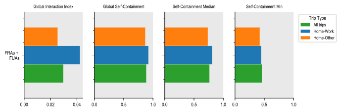
Note: OECD computations based on KOTI mobile phone data. The input data is mobile phone (cell-tower-based) data at municipal level. These figures were computed for a typical work week (7 to 13 November 2022) and a holiday week (8 to 12 September 2022).
The analysis then compares LMAs with FRAs and FUAs in Japan and Australia. Australia’s official Working Zones (WZs) (Australian Government, 2023[2]) and Japan’s Commuting Zones (CZs) (Research Institute of Economy, 2021[3]) provide the reference LMA delineations. Because the measures are affected by the number and average size of the units being compared, the FRA parameters are calibrated to produce a total number of FRAs and FUAs as close as possible to the number of LMAs.
Japan has 265 LMAs covering its entire territory. The FRA configuration based on driving-time thresholds of 30 minutes and 120 minutes for catchment areas below 25 000 inhabitants yields 203 FRAs. Evaluating them jointly with the 61 Japanese FUAs matches almost exactly the number of LMAs, which allows for an accurate comparison between these two delineations of daily systems.
In Japan, both LMAs and FRAs + FUAs present broadly similar levels of autonomy and cohesion for work-related and non-work trips alike (Figure 4.10 and Figure 4.11). For LMAs, distinguishing between work and non-work trips primarily affects the global interaction index and the minimum self-containment; for FRAs + FUAs the strongest effect is on the global interaction index. FRAs + FUAs show somewhat higher global self-containment and minimum self-containment than LMAs, while LMAs exhibit a somewhat higher global interaction index. Median self-containment is almost equal in both delineations. This suggests that the overall incidence of cross-boundary flows between daily systems is comparable between the two delineations. LMAs are somewhat more homogeneous than FRAs + FUAs in terms of population size and slightly more homogeneous when considering their area.
Autonomy and cohesion metrics obtained for LMAs and FRAs + FUAs in Japan
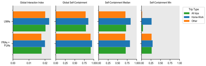
Note: OECD computations based on Habidatum mobile phone data.
Homogeneity metrics obtained for LMAs and FRAs + FUAs in Japan
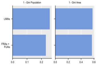
Note: OECD computations based on Habidatum mobile phone data.
Australia has 313 LMAs and 18 FUAs. The FRA configuration examined here results in 251 FRAs, yielding the closest match between the number of FRAs + FUAs and LMAs. It relies on driving-time thresholds of 15 minutes and 30 minutes for catchment areas below 25 000 inhabitants.
Australian LMAs and FRAs + FUAs also show overall similar levels of autonomy and cohesion (Figure 4.12). The global interaction index and global self-containment are almost equal in both delineations, whether considering work or non-work trips. For both LMAs and FRAs + FUAs, distinguishing between work and non-work trips primarily affects the global interaction index. FRAs + FUAs show slightly higher median self-containment and minimum self-containment. It is noteworthy that a higher number of daily systems (as for the LMAs in this example) tends to yield lower self-containment and higher cohesion values. For LMAs, the difference in median self-containment between home-work trips and other trips is slightly higher than for FRAs + FUAs. LMAs are slightly more homogeneous when considering their geographic size, whereas FRAs + FUAs are more homogeneous when considering the population living in the daily systems (Figure 4.13).
Autonomy and cohesion metrics obtained for LMAs and FRAs + FUAs in Australia
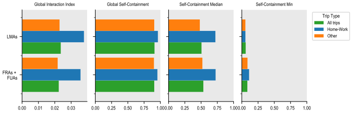
Note: OECD computations based on Habidatum mobile phone data.
Homogeneity metrics obtained for LMAs and FRAs + FUAs in Australia
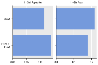
Note: OECD computations based on Habidatum mobile phone data.
Taken together, the results for Australia, Japan and Korea suggest that FRA-FUA boundaries capture similar shares of work-related and other mobility. Differences by trip purpose are more apparent in the internal structure of mobility: work trips more often connect different municipalities within the same functional area, while other trips are either more local or more likely to cross its boundaries. The close comparison with LMAs in Japan also indicates that FRAs and FUAs can represent mobility patterns beyond commuting, even though observed flows are not used to delineate FRAs. The Australian findings point in the same direction and are broadly consistent with those for Japan, although the remaining difference in the number of units under the two delineations should still be considered when interpreting the results.
References
[2] Australian Government, D. (2023), Working zones update, https://www.infrastructure.gov.au/department/media/publications/working-zones-update.
[1] Martínez-Bernabeu, L., M. Coombes and J. Casado-Díaz (2019), “Functional Regions for Policy: a Statistical ‘Toolbox’ Providing Evidence for Decisions between Alternative Geographies”, Applied Spatial Analysis and Policy, Vol. 13/3, pp. 739-758, https://doi.org/10.1007/s12061-019-09326-2.
[3] Research Institute of Economy, T. (2021), RIETI - Commuting zones in Japan, https://www.rieti.go.jp/en/columns/v01_0152.htm.
← 1. A stay point is the location where a device remains within a small geographic area for a minimum period of time, indicating that the user has stopped rather than simply passed through.
← 2. It is possible to measure population size through mobile phone data. However, Habidatum scales the mobile phone users by the census population.